This work is part of a joint project with Staffordshire University. It wouldn’t have been possible without the help of Claire Gwinnett, Andrew Jackson, Jolien Casteele, Zoe Jones and Mohamed Sedky.

---

“Every contact leaves a trace” - (a paraphrase of) Locard’s exchange principle

Whenever you touch anything - anything - you leave some evidence behind and take some evidence with you. When it comes to contact with cloth, that might come in the form of fibres that transfer between surfaces. In Forensic Science, “persistence and transfer” studies aim to discover the mechanics of this. These studies typically involve manually counting fluorescent fibres under magnification.

This blog post introduces a prototype Neural Network-based model for counting the fibres automatically - to speed experiments up and make results more easily reproducible. I focussed on fibres ‘lifted’ from surfaces with sticky tape. Running on a GPU, the model can count fibres in a 12cm x 5cm area in ~3-6 seconds.

The code for the project can be found here.

The model’s smarts

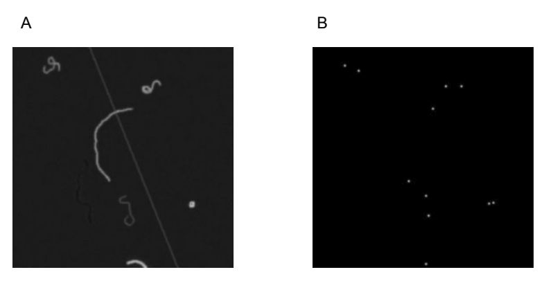
The prototype uses a Convolutional Neural Network (CNN), which is trained to produce an estimated density map from a fibre image. Rather than the model directly estimating of the number of fibres, the density map shows where the model thinks the ends of each fibre are, with each end labelled with a blurred dot (Figure 2). The ‘area under’ each dot is approximately 1, so (assuming each fibre has two detectable ends) the total number of fibres can be estimated by sum(density_map) / 2.

CNNs are adept at recognising structure, with the rough distances between relative elements suggesting what an object is. In a way, a fibre is the antithesis of this. If you look at a portion of a fibre, it’s very difficult to predict what the rest of it is going to do; much more challenging than with people or cells. I considered fibre ends the best candidate for detection with CNNs for this reason.

In a 2015 paper, Xie et. al. showed that CNNs could be used to produce density maps that yielded effective estimates the number of fluorescent cells in a slide; achieving an absolute mean error of 3.2 (with a standard deviation of 0.2) on images containing 174±64 cells. In particular, Xie used a ‘Fully Convolutional Regression Network’ (FCRN) architecture - a Neural Network where every layer is convolutional.

For the prototype to be practically useful, it needs to able to work on fairly large images (~3500 x 1500 pixels), but in training it to be shown many smaller examples (e.g. 64 x 64 pixels). This is made easier by FCRNs, since convolutional layers can be adapted to work on inputs of arbitrary size:

“[An FCRN] can take an input of arbitrary size and produce a correspondingly-sized output both for end-to-end training and for inference.” - Xie et. al

No re-training or post-processing needs to occur to resize the model.

Getting hold of training data

With a model in place, I needed to find well-labelled data to train it on. Perhaps Neural Networks’ biggest downside is how data-hungry they tend to be. The model needs to see 1000s of examples to learn well. Finding and annotating that number of real-world fluorescent fibre images is a daunting task. To make quick progress on the project, I programmatically generated the data, giving us a virtually unlimited supply of training examples.

It comes at a cost, though. You can only expect a model trained on this data to be good at generalising to real-world situations if the data are well designed.

In this case, that involved looking closely at the characteristics of real world examples and attempting to faithfully replicate them in the programmatic version. Those characteristics include not only the inherent properties of fibres - curliness, thickness & brightness - but also artefacts common in images of fibre lifts - tape edges refracting light, imperfect camera focus & trapped air-bubbles.

In a supervised learning problem like this, you need both the training images and a label. In this case, the labels are density maps showing where the fibre ends really are (Figure 2).

Quieting the noise

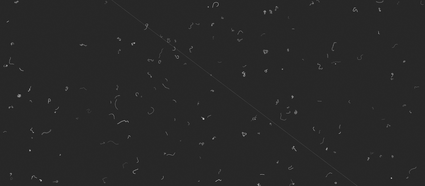
While the model appeared to be learning well during training, it struggled when facing more realistic programmatically generated images. Given the image in Figure 4, the model predicted it contained -7746.135 fibres… a clear sign something was up.

After investigation, it was clear that the sheer sparseness of fibre ends in the image was the issue. Most pixels in the density map were meant to represent non-fibre-ends; ideally, we’d like these to be 0 exactly.

The model was trained using an L2 loss function (a pixel-wise mean-squared-error) which incentivises the model to get close to the correct value, but doesn’t punish minor variations. These variations in the density map for what should have been ‘dead space’ added up over millions of pixels; leading to enough noise to drown out the signal.

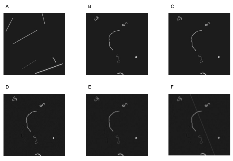
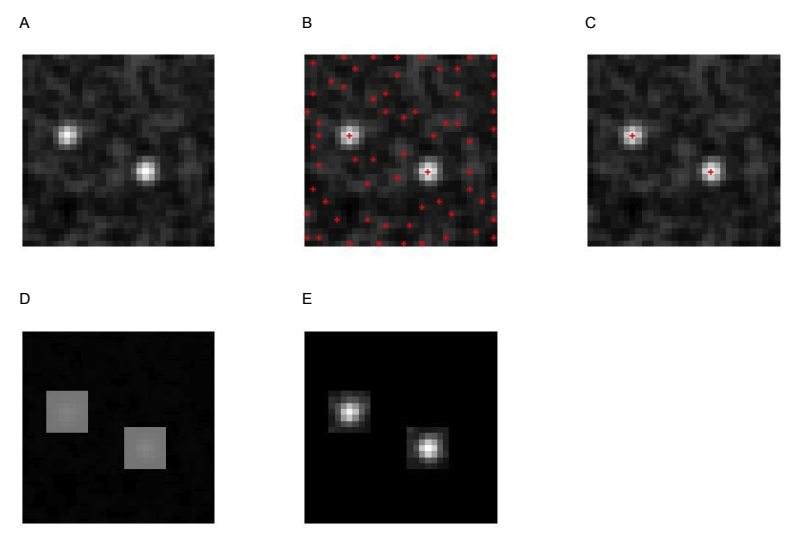
To cut back the noise, I decided to find the locations of obvious fibre ends in the density map and only count pixels in the immediate area; a process I called ‘Peak Masking’ in the code. Figure 5 shows the steps in the algorithm:

Given a density map (A), find all pixels that are ‘peaks’ (larger than their immediate neighbours) (B). Filter out all peaks under a given threshold (C), create squares centred on the remaining peaks (D) and use the squares as a mask to remove the majority of the noise (E).

The Peak Masking algorithm has two parameters - the threshold a peak must pass to be kept, and the size of the surrounding area to keep. Rather than twiddle with these parameters myself, I used hyperopt to find the optimal values. To make sure that this approach didn’t slow down the evaluation too much, I implemented it in tensorflow.

With Peak Masking, the model estimated a much-more-reasonable 155.96965 (compared to the real count of 169).

Obtaining real data

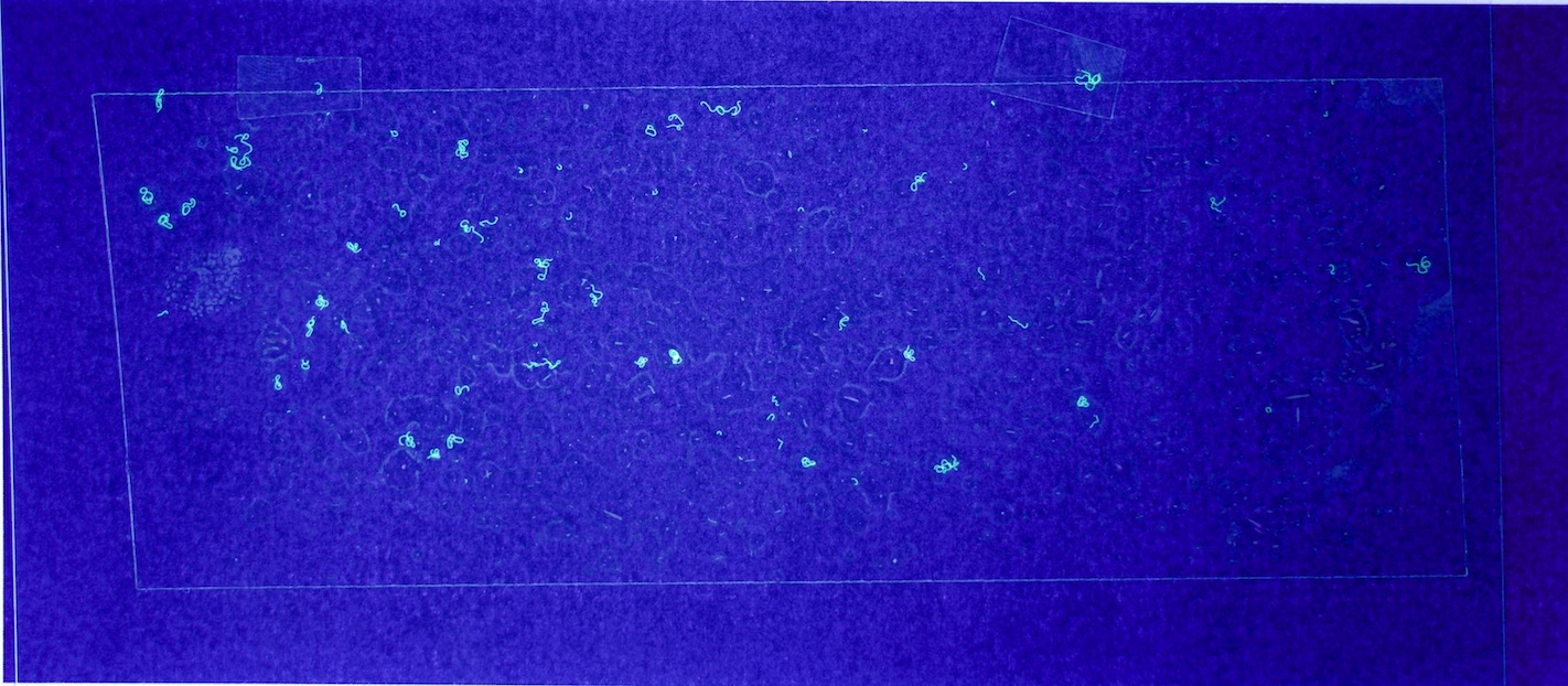
For this prototype to demonstrate that using machine learning for fibre counting might be practical in research, the process of getting data into the model needs to be as automated as possible; and use relatively common equipment. In my case, that means a mid-range DSLR camera, a UV torch, and a printer. Using Aruco markers to correct perspective made the process tolerant to variations in set-up.

Figures 6.a-d. show how a raw image taken with this equipment gets pre-processed for use with the model.

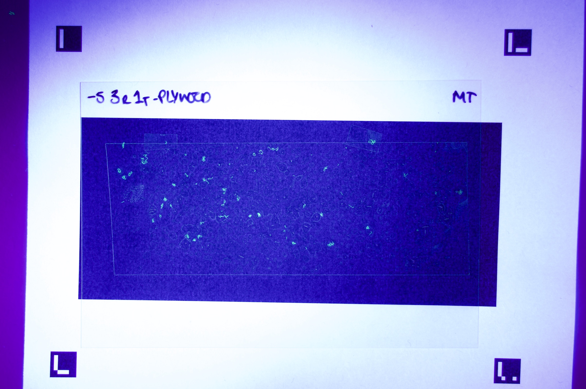
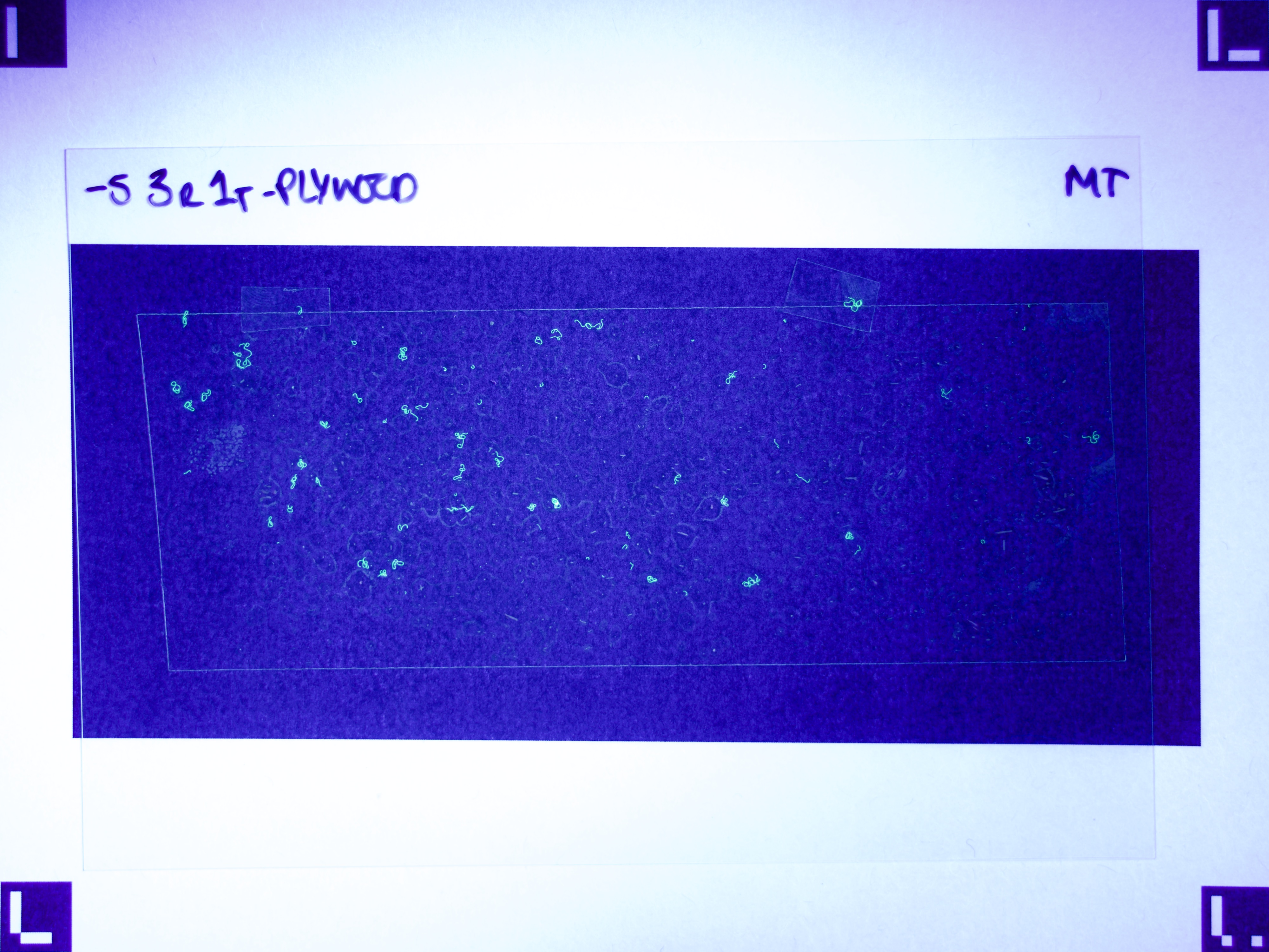
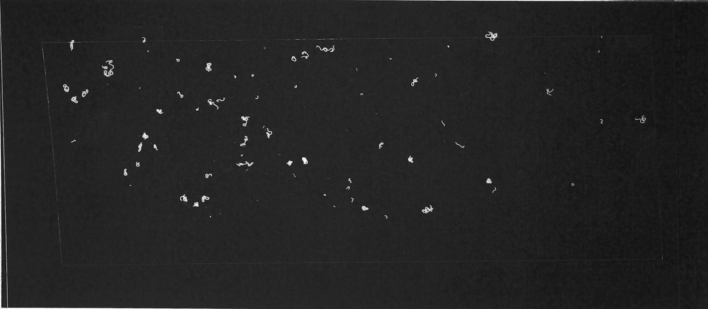
The step shown in Figure 6.d is particularly important, since by changing the parameters of the pre-processing script, you can count fibres of any distinct colour you choose.

As important as low cost is practicality; is it really faster to take these images and let a computer produce a count than manually counting them yourself? Happily, with a little practice, in the region of 100s of these images can be produced in an hour. A fuller guide can be found here.

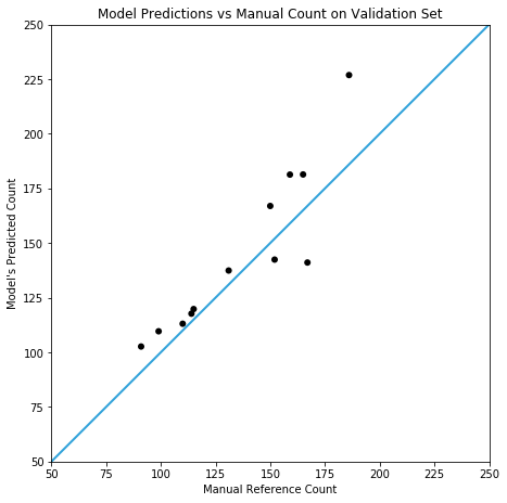
Results

Testing against a (small) real world validation set, you can see the prototype is somewhat accurate, but it doesn’t yet compare with the results in cell counting reported by Xie et. al. In this case, the model achieves a mean absolute error of 14.3 (with a standard deviation of 11.0) on slides containing 138±48 fibres.

Conclusion

This prototype represents a decent first step towards the eventual goal of automated fluorescent fibre counting; but there are clearly some improvements still on the table. I suspect that a combination of fine-tuning the model (against manually labelled real world data) and using it in an ensemble with a complementary model (e.g. using YOLO or Mask-RCNN to detect corner cases) would yield the best improvements.